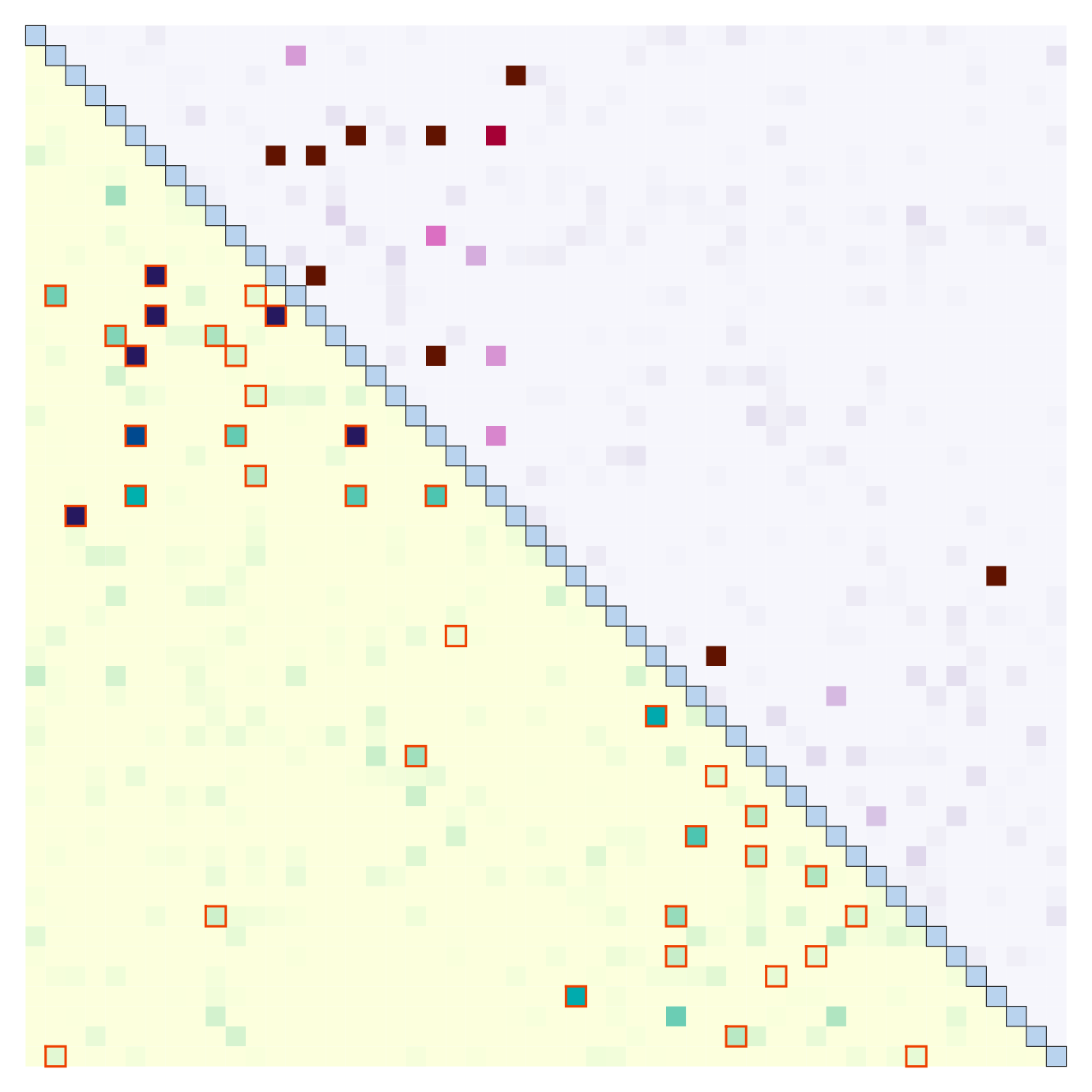
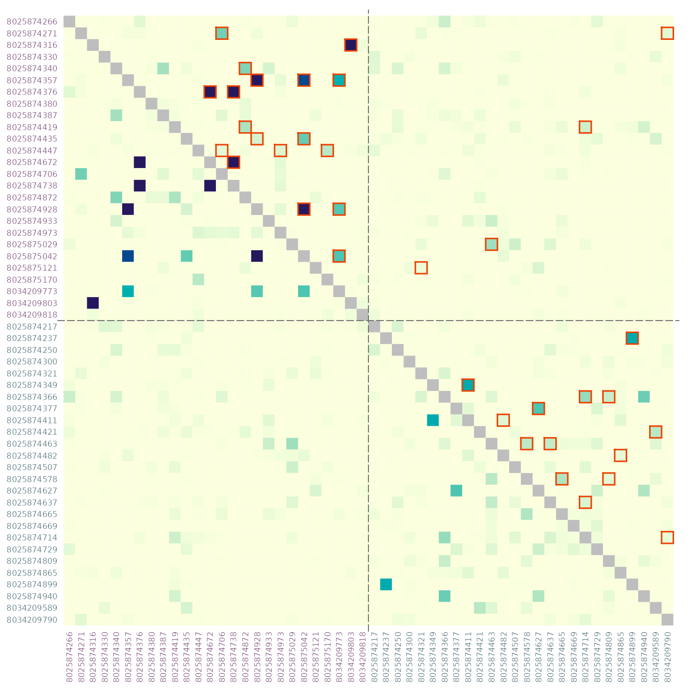
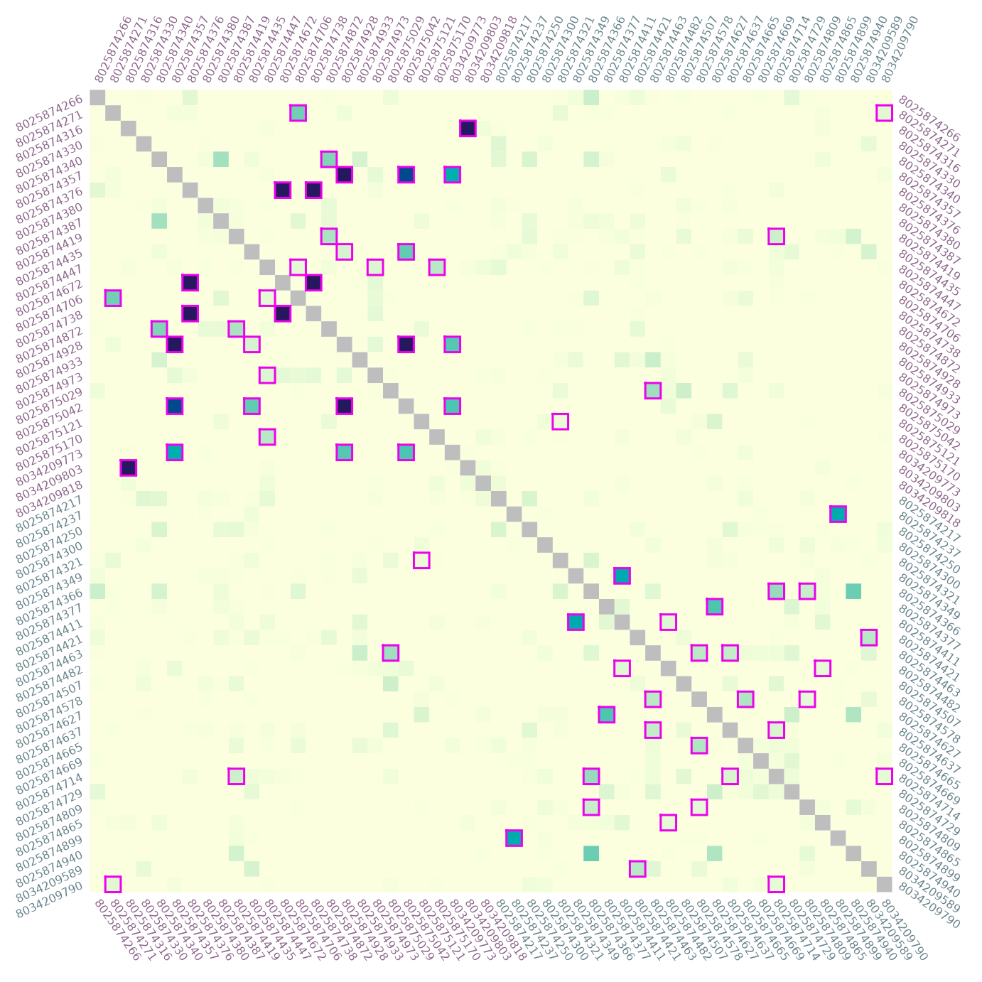
Represents a matrix of pairwise relatedness estimates with colors corresponding to the levels of relatedness. Optionally, also outlines results of a hypothesis testing. The plot follows a matrix layout.
Usage
plotRel(
  r,
  rlim = c(0, 1),
  sig = NULL,
  alpha = NULL,
  col = grDevices::hcl.colors(101, "YlGnBu", rev = TRUE),
  draw_diag = FALSE,
  col_diag = "gray",
  border_diag = NA,
  lwd_diag = 0.5,
  border_sig = "orangered2",
  lwd_sig = 1.5,
  xlab = "",
  ylab = "",
  add = FALSE,
  idlab = FALSE,
  side_id = c(1, 2),
  col_id = 1,
  cex_id = 0.5,
  srt_id = NULL,
  ...
)
Arguments
- r
a matrix or a 3-dimensional array as returned by
ibdDat.- rlim
the range of values for colors. If
NULLorNA, will be calculated fromr.- sig
a logical matrix specifying which entries of the relatedness matrix should be outlined or "amplified" (made larger).
sigtakes precedence overalpha.- alpha
significance level for hypothesis testing; determines relatedness matrix entries to be outlined. Ignored if
sigis notNULL.- col
the colors for the range of relatedness values.
- draw_diag
a logical value specifying if diagonal cells should be distinguished from others by a separate color.
- col_diag, border_diag, lwd_diag
the color for the fill, the color for the border, and the line width for the border of diagonal entries. Ignored if
draw_diag = FALSE.- border_sig, lwd_sig
the color and the line width for outlining entries specified by
sigoralpha. Ifborder_sigisNA, these entries will be "amplified", their size controlled bylwd_sig.- xlab, ylab
axis labels.
- add
a logical value specifying if the graphics should be added to the existing plot (useful for triangular matrices).
- idlab
a logical value specifying if sample ID's should be displayed.
- side_id
an integer vector specifying plot sides for sample ID labels.
- col_id, cex_id
numeric vectors for the color and the size of sample ID labels.
- srt_id
a vector of the same length as
side_idspecifying rotation angles for sample ID labels. IfNULL, the labels will be perpendicular to the axes.- ...
other graphical parameters.
See also
plotColorbar for a colorbar and mixMat
for combining square matrces.
Examples
parstart <- par(no.readonly = TRUE)   # save starting graphical parameters

par(mar = c(0.5, 0.5, 0.5, 0.5))
plotRel(dres, alpha = 0.05, draw_diag = TRUE)

# draw log of p-values in the upper triangle
pmat <- t(log(dres[, , "p_value"]))
pmat[pmat == -Inf] <- min(pmat[is.finite(pmat)])
plotRel(pmat, rlim = NULL, draw_diag = TRUE, col = hcl.colors(101, "PuRd"),
        add = TRUE, col_diag = "slategray2", border_diag = 1)


# symmetric matrix, outline significant in upper triangle, display sample ID
par(mar = c(3, 3, 0.5, 0.5))
dmat  <- dres[, , "estimate"]
dmats <- mixMat(dmat, dmat)
sig <- dres[, , "p_value"] <= 0.05
col_id <- rep(c("orchid4", "cadetblue4"), each = 26)
plotRel(dmats, sig = t(sig), border_sig = "magenta2", draw_diag = TRUE,
        idlab = TRUE, col_id = col_id)
abline(v = 26, h = 26, col = "gray45", lty = 5)


# rotate sample ID labels on all sides, increase size for significant pairs
par(mar = c(3, 3, 3, 3))
sig <- dres[, , "p_value"] <= 0.01
plotRel(dmats, sig = mixMat(sig, sig), border_sig = NA, lwd_sig = 5,
        draw_diag = TRUE, idlab = TRUE, side_id = 1:4, col_id = col_id,
        srt_id = c(-55, 25, 65, -35))

par(parstart)