Package dcifer (Distance for Complex Infections: Fast Estimation of Relatedness) calculates genetic distance between polyclonal infections by estimating relatedness from biallelic and multiallelic data [1]. In addition to estimates, the package provides a likelihood function and statistical inference. Functions for reading and reformatting data, performing preparatory steps, and visualizing the results are also included. We will illustrate the analysis process using microhaplotype data from two health facilities in Maputo and Inhambane provinces of Mozambique [2].

You can install the released version of dcifer from CRAN with:
install.packages("dcifer")and the development version from GitHub with:
# install.packages("remotes")
remotes::install_github("EPPIcenter/dcifer")
# or, to include a vignette:
remotes::install_github("EPPIcenter/dcifer", build_vignettes = TRUE)
library(dcifer)
help(package = "dcifer")
vignette(package = "dcifer", "vignetteDcifer")
pardef <- par(no.readonly = TRUE)
Read and reformat data, estimate COI and population allele frequencies
Dcifer relatedness estimation requires sample data in a specific format as well as estimates of complexity of infection (COI) and population allele frequencies. Here is an example of some preparation steps using Mozambique dataset. First, read in original data stored in a .csv file in a long format.
| sampleID | locus | allele | clinic | province |
|---|---|---|---|---|
| 8025874217 | t1 | HB3.0 | Inhassoro | Inhambane |
| 8025874217 | t1 | D10–D6–FCR3–V1-S.0 | Inhassoro | Inhambane |
| 8025874217 | t20 | U659.0 | Inhassoro | Inhambane |
The name of the file is the first argument to the function that reads and reformats the data:
sfile <- system.file("extdata", "MozParagon.csv", package = "dcifer")
dsmp <- readDat(sfile, svar = "sampleID", lvar = "locus", avar = "allele")
str(dsmp, list.len = 2)
#> List of 52
#>  $ 8025874217:List of 87
#>   ..$ t1  : Named num [1:5] 1 1 0 0 0
#>   .. ..- attr(*, "names")= chr [1:5] "D10--D6--FCR3--V1-S.0" "HB3.0" "t1.0" "t1.1" ...
#>   ..$ t10 : Named num [1:4] 1 0 0 0
#>   .. ..- attr(*, "names")= chr [1:4] "D10--D6--HB3.0" "t10.0" "t10.2" "U659.0"
#>   .. [list output truncated]
#>  $ 8025874237:List of 87
#>   ..$ t1  : Named num [1:5] 0 0 0 0 1
#>   .. ..- attr(*, "names")= chr [1:5] "D10--D6--FCR3--V1-S.0" "HB3.0" "t1.0" "t1.1" ...
#>   ..$ t10 : Named num [1:4] 1 0 0 0
#>   .. ..- attr(*, "names")= chr [1:4] "D10--D6--HB3.0" "t10.0" "t10.2" "U659.0"
#>   .. [list output truncated]
#>   [list output truncated]
Or, to reformat an R data frame (dlong) containing the same dataset:
dsmp <- formatDat(dlong, svar = "sampleID", lvar = "locus", avar = "allele")
# optionally, extract location information
meta <- unique(read.csv(sfile)[c("sampleID", "province")])
meta <- meta[match(names(dsmp), meta$sampleID), ]  # order samples as in dsmp
Next, estimate COI for all the samples - here we use naive estimation, first ranking loci of a sample by the number of detected alleles, and then using a locus with a prescribed rank (lrank) to determine COI:
lrank <- 2
coi   <- getCOI(dsmp, lrank = lrank)
Finally, estimate population allele frequencies, adjusting for COI:
afreq <- calcAfreq(dsmp, coi, tol = 1e-5)
str(afreq, list.len = 2)
#> List of 87
#>  $ t1  : Named num [1:5] 0.4239 0.2808 0.1116 0.0422 0.1415
#>   ..- attr(*, "names")= chr [1:5] "D10--D6--FCR3--V1-S.0" "HB3.0" "t1.0" "t1.1" ...
#>  $ t10 : Named num [1:4] 0.8539 0.00942 0.00951 0.12717
#>   ..- attr(*, "names")= chr [1:4] "D10--D6--HB3.0" "t10.0" "t10.2" "U659.0"
#>   [list output truncated]
In some situations, population allele frequencies might be estimated from a different (e.g. larger) dataset and provided separately (e.g. in a .csv file or R data frame):
| locus | allele | freq |
|---|---|---|
| t1 | D10–D6–FCR3–V1-S.0 | 0.44377920 |
| t1 | HB3.0 | 0.27713450 |
| t1 | t1.0 | 0.09375438 |
In that case, after the frequencies are read in, they need to be checked against the the existing data object to make sure that all the loci and alleles are in the same order. Function matchAfreq performs the checking and provides updated matching sample data and allele frequencies. For that procedure, loci and alleles in both lists (dsmp and afreq) have to be named; otherwise the names are not required, and the order of loci and alleles is assumed to be the same for sample data and allele frequencies. If afreq contains “extra” alleles that are not listed in dsmp, these alleles are added to dsmp. If dsmp has alleles not included in afreq or listed with a frequency of 0, they are assigned a small probability (optional minfreq argument) with subsequent renormalization.
afile  <- system.file("extdata", "MozAfreq.csv", package = "dcifer")
afreq2 <- readAfreq(afile, lvar = "locus", avar = "allele", fvar = "freq")
# alternatively, if allele frequencies are provided in an R data frame (aflong):
afreq2 <- formatAfreq(aflong, lvar = "locus", avar = "allele", fvar = "freq")
da_upd <- matchAfreq(dsmp, afreq2, minfreq = 1/sum(coi)/10)
dsmp2  <- da_upd$dsmp
afreq2 <- da_upd$afreq
Estimate relatedness
As a first step in relatedness estimation, we set (only one pair of strains between two infections can be related) and test the hypothesis that infections are unrelated (). This is done with ibdDat function. Then we explore significantly related pairs in more detail.
For the purposes of demonstration, we first estimate relatedness and display results using dsmp as created previously where samples are not sorted by location.
dres0 <- ibdDat(dsmp, coi, afreq, pval = TRUE, confint = TRUE, rnull = 0,
                alpha = 0.05, nr = 1e3)
Look at the results for a single pair of samples:
dres0[17, 10, ]
#>   estimate    p_value   CI_lower   CI_upper
#> 0.31000000 0.06255194 0.00000000 0.67900000
Alternatively, we may want to first sort samples by clinic or geographic location:
provinces <- c("Maputo", "Inhambane")
nsite     <- table(meta$province)[provinces]
ord       <- order(factor(meta$province, levels = provinces))
dsmp <- dsmp[ord]
coi  <- coi[ ord]
dres <- ibdDat(dsmp, coi, afreq) To test different hypotheses, we can use rnull and side arguments. For example, to test whether pairwise relatedness is higher than 0.2 () and obtain one-tailed p-values:
dres_hi <- ibdDat(dsmp, coi, afreq, rnull = 0.2, side = "right")Visualize the results
When pairwise relatedness is calculated within a single dataset, ibdDat returns triangular matrices. For plotting, we can make them symmetric. Then significantly related pairs can be outlined in either or both triangles.
Display the results for unsorted samples, with sample ID’s written on the margins. Label colors correspond to locations (health facilities):
par(mar = c(3, 3, 1, 1))
alpha <- 0.05                          # significance level
dmat <- dres0[, , "estimate"]
# create symmetric matrix
dmat <- mixMat(dmat, dmat)
# determine significant, highlight them in the upper triangle
sig <- dres0[, , "p_value"] <= alpha
plotRel(dmat, sig = t(sig), draw_diag = TRUE, lwd_diag = 0.5, idlab = TRUE,
col_id = c(3:4)[factor(meta$province)]) 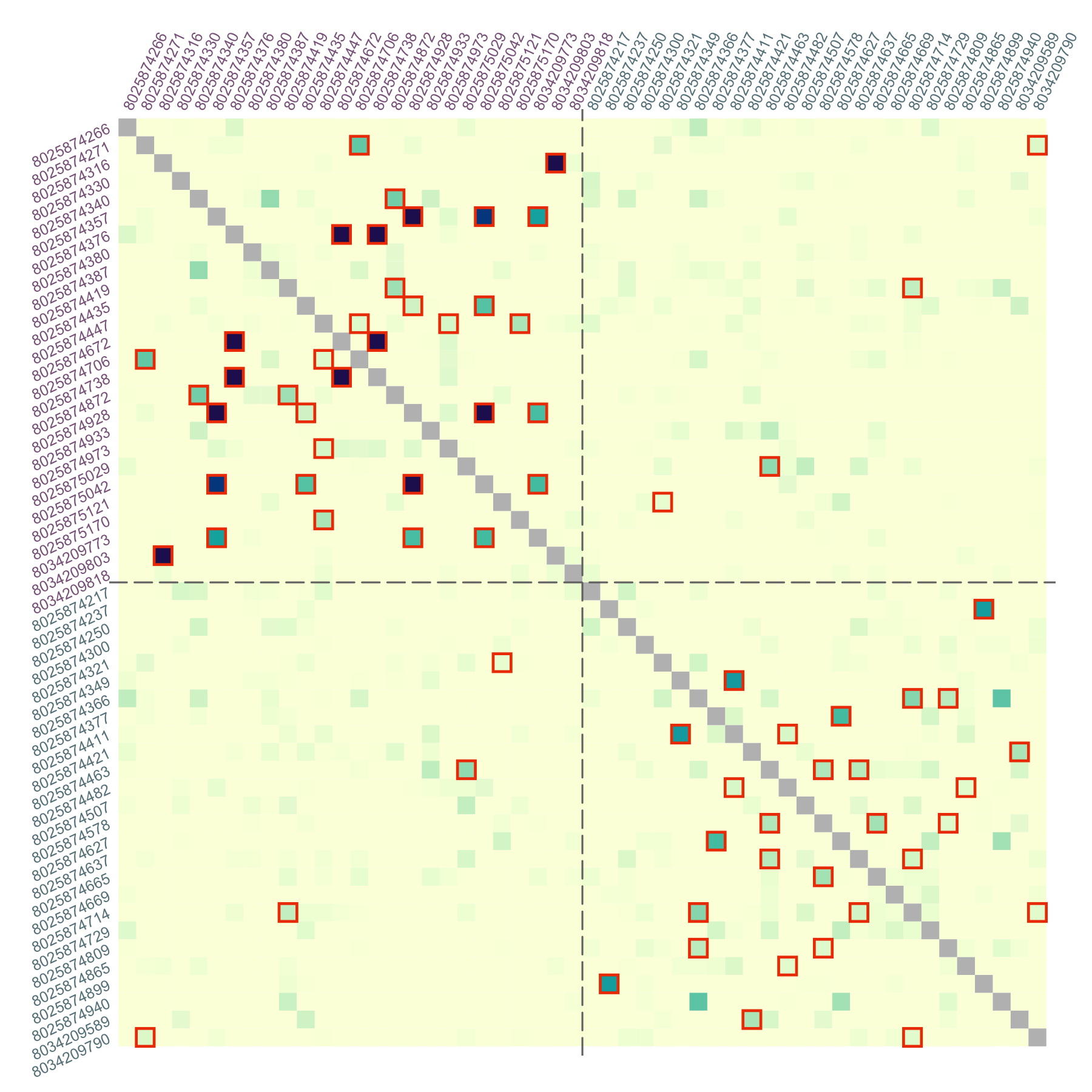
For the sorted samples:
par(mar = c(1, 3, 3, 1))
nsmp  <- length(dsmp)
atsep <- cumsum(nsite)[-length(nsite)]
dmat  <- dres[, , "estimate"]
dmat  <- mixMat(dmat, dmat)
sig   <- dres[, , "p_value"] <= alpha
col_id <- rep(c("orchid4", "cadetblue4"), nsite)
plotRel(dmat, sig = mixMat(sig, sig), draw_diag = TRUE, idlab = TRUE,
        side_id = c(2, 3), col_id = col_id, srt_id = c(25, 65))
abline(v = atsep, h = atsep, col = "gray45", lty = 5)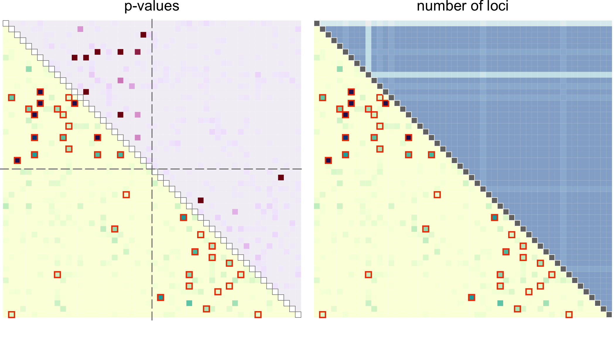
When the number of samples is large, individual pairs can be hard to see. To make relatedness structure more visible, significantly related pairs can be “amplified”, or made larger:
par(mfrow = c(1, 4), mar = c(0.5, 0.5, 0.5, 0.5))
sig_hi <- dres_hi[, , "p_value"] <= alpha
sigsym <- mixMat(sig_hi, sig_hi)
plotRel(dmat, sig = sigsym, draw_diag = TRUE, lwd_sig = 0)
abline(v = atsep, h = atsep, col = "gray45", lty = 5)       # no highlighting
plotRel(dmat, sig = sigsym, draw_diag = TRUE, lwd_sig = 2)
abline(v = atsep, h = atsep, col = "gray45", lty = 5)       # outline
plotRel(dmat, sig = sigsym, draw_diag = TRUE, border_sig = NA, lwd_sig = 1.5)
abline(v = atsep, h = atsep, col = "gray45", lty = 5)       # amplification
plotRel(dmat, sig = sigsym, draw_diag = TRUE, border_sig = NA, lwd_sig = 2.5)
abline(v = atsep, h = atsep, col = "gray45", lty = 5)       # more amplification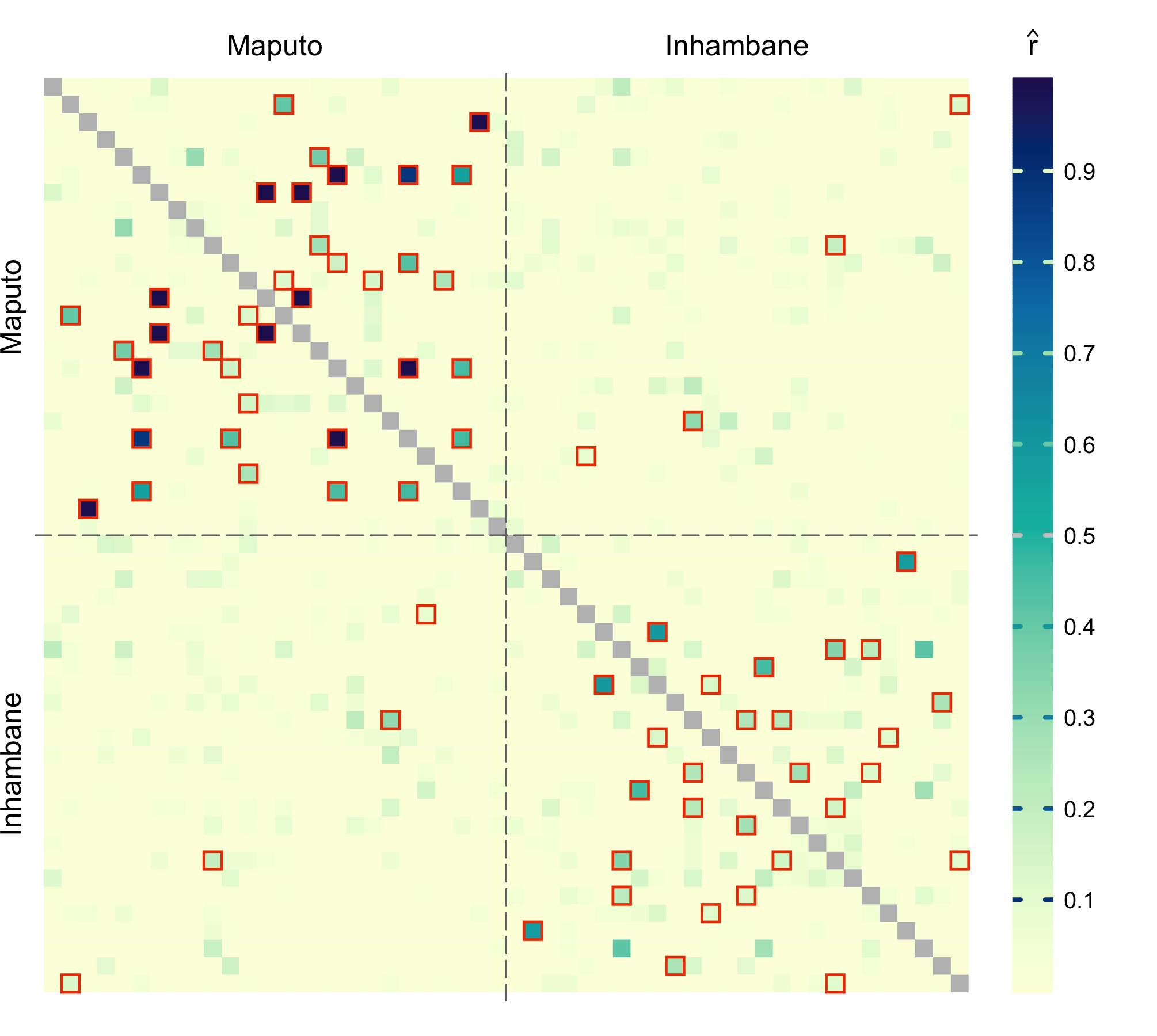
par(pardef)For these symmetric distance measures, one of the triangles can be used to display other relevant information, such as p-values, geographic distance, or a number of non-missing loci between two samples. For that, use add = TRUE.
par(mfrow = c(1, 2), mar = c(1, 0, 1, 0.2))
plotRel(dres, draw_diag = TRUE, alpha = alpha)
mtext("p-values", 3, 0.2)
# p-values for upper triangle
pmat <- t(log(dres[, , "p_value"]))
pmat[pmat == -Inf] <- min(pmat[is.finite(pmat)])
plotRel(pmat, rlim = NULL, draw_diag = TRUE, col = hcl.colors(101, "Red-Purple"),
        add = TRUE, col_diag = "white", border_diag = "gray45")
abline(v = atsep, h = atsep, col = "gray45", lty = 5)

# number of non-missing loci for upper triangle
dmiss <- lapply(dsmp, function(lst) sapply(lst, function(v) all(!v)))
nmat <- matrix(NA, nsmp, nsmp)
for (jsmp in 2:nsmp) {
  for (ismp in 1:(jsmp - 1)) {
    nmat[ismp, jsmp] <- sum(!dmiss[[ismp]] & !dmiss[[jsmp]])
  }
}
nrng <- range(nmat, na.rm = TRUE)
par(mar = c(1, 0.2, 1, 0))
plotRel(dres, draw_diag = TRUE, alpha = alpha)
mtext("number of loci", 3, 0.2)
coln <- hcl.colors(diff(nrng)*2.4, "Purple-Blue", rev = TRUE)[1:(diff(nrng) + 1)]
plotRel(nmat, rlim = NA, col = coln, add = TRUE, draw_diag = TRUE,
        col_diag = "gray45", border_diag = "white")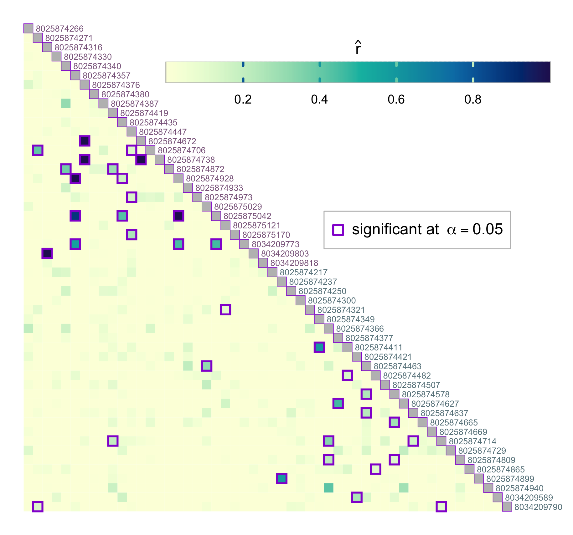
par(pardef)For reference, add a colorbar legend to the plot. It can be placed beside the main plot. For the upper matrix, we outline the pairs for which relatedness is significantly higher than (at the same significance level ):
layout(matrix(1:2, 1), width = c(7, 1))
par(mar = c(1, 1, 2, 1))
sig_hi <- dres_hi[, , "p_value"] <= alpha  #*** out here, not in vignette!!!
plotRel(dmat, sig = mixMat(sig, sig_hi), draw_diag = TRUE)
atclin <- cumsum(nsite) - nsite/2
abline(v = atsep, h = atsep, col = "gray45", lty = 5)
mtext(provinces, side = 3, at = atclin, line = 0.2)
mtext(provinces, side = 2, at = atclin, line = 0.2)
par(mar = c(1, 0, 2, 3))
plotColorbar()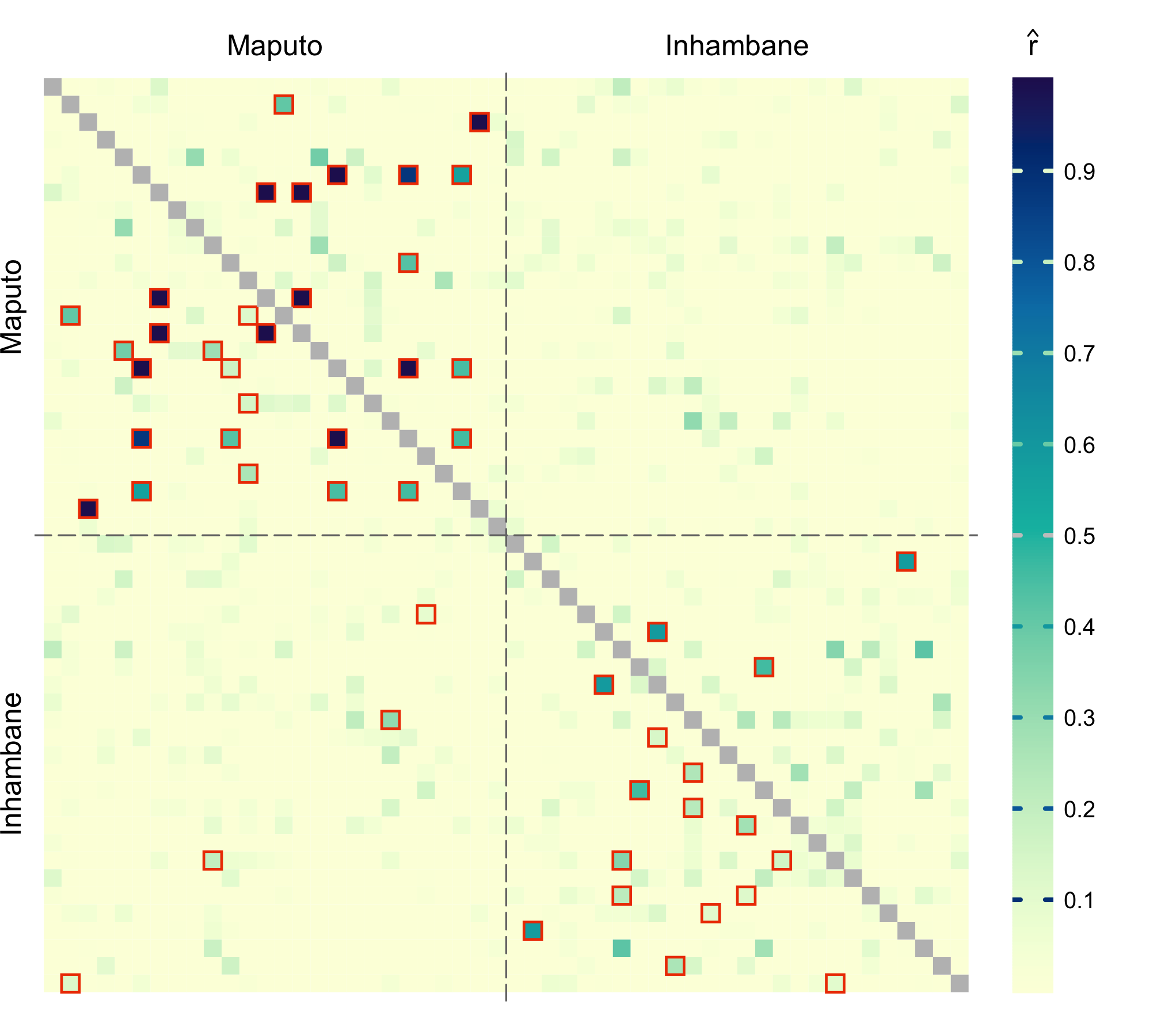
par(pardef)The colorbar can also be located in the empty space left by the triangular matrix. In the example below, we specify horizontal colorbar and provide custom tick mark locations:
# horizontal colorbar
par(mar = c(1, 1, 1, 3))
border_sig <- "darkviolet"
plotRel(dres, draw_diag = TRUE, border_diag = border_sig, alpha = alpha,
        border_sig = border_sig, lwd_sig = 2)
legend(32, 20, pch = 0, col = border_sig, pt.lwd = 2, pt.cex = 1.4,
       box.col = "gray", legend = expression("significant at" ~~ alpha == 0.05))
text(1:nsmp + 0.3, 1:nsmp - 0.5, labels = names(dsmp), col = col_id, adj = 0,
     cex = 0.55, xpd = TRUE)
par(fig = c(0.25, 1, 0.81, 0.92), mar = c(1, 1, 1, 1), new = TRUE)
plotColorbar(at = c(0.2, 0.4, 0.6, 0.8), horiz = TRUE)
ncol <- 301
lines(c(0, ncol, ncol, 0, 0), c(0, 0, 1, 1, 0), col = "gray")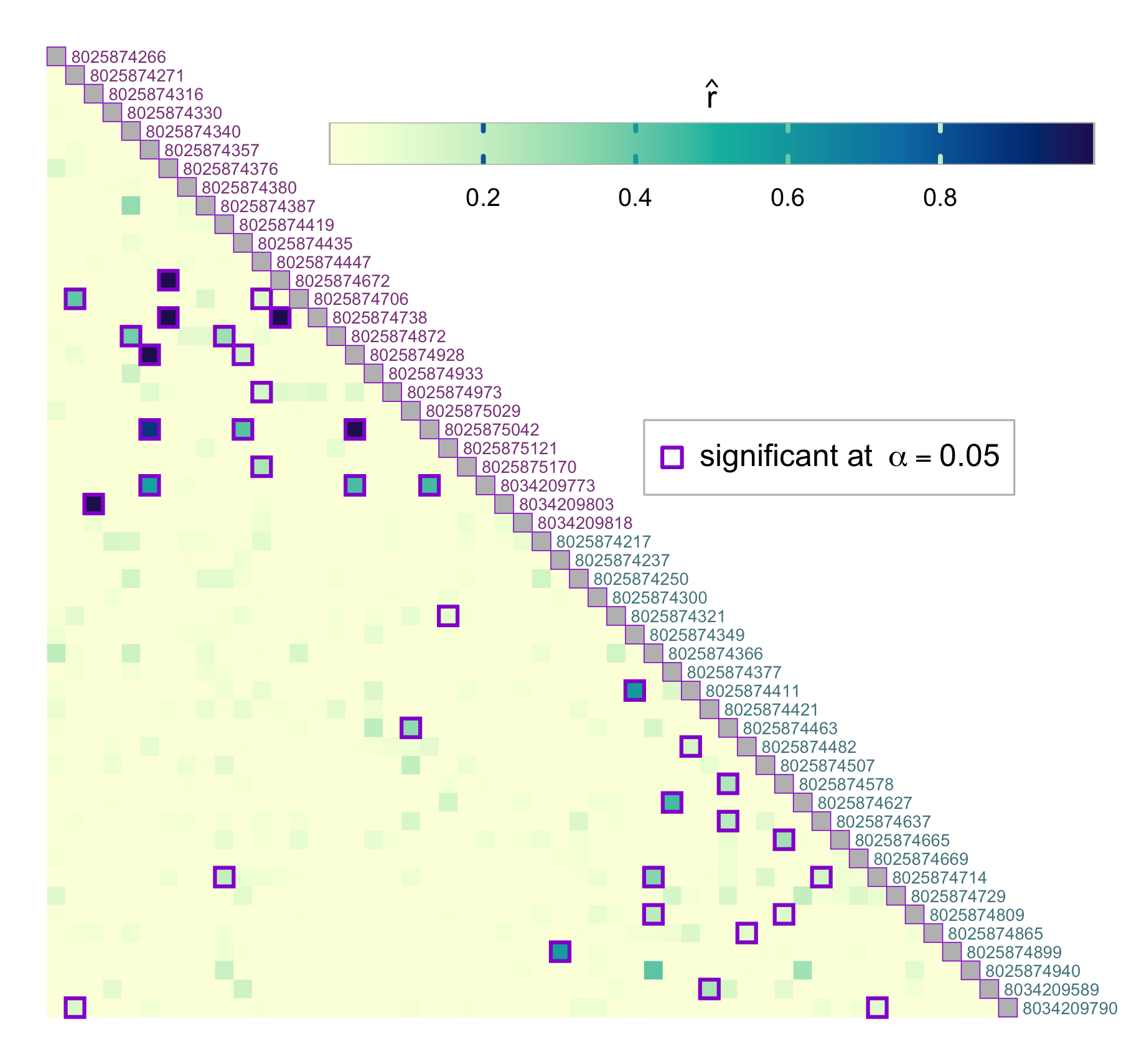
par(pardef)Further analysis of related samples
Examine pairs that are determined to be significantly related at the significance level more closely by allowing multiple pairs of strains to be related between two infections. Using ibdEstM, we also estimate the number of positively related pairs of strains and compare results yielded by a constrained model assuming (faster method) and without the constraint. In addition, we look at the estimates of overall relatedness.
# First, create a grid of r values to evaluate over
revals <- mapply(generateReval, 1:5, nr = c(1e3, 1e2, 32, 16, 12))
isig <- which(sig, arr.ind = TRUE)
nsig <- nrow(isig)
sig1 <- sig2 <- vector("list", nsig)
for (i in 1:nsig) {
  sig1[[i]] <- ibdEstM(dsmp[isig[i, ]], coi[isig[i, ]], afreq, Mmax = 5,
                       equalr = FALSE, reval = revals)
}
for (i in 1:nsig) {
  sig2[[i]] <- ibdEstM(dsmp[isig[i, ]], coi[isig[i, ]], afreq, equalr = TRUE)
}
M1      <- sapply(sig1, function(r) sum(r > 0))
M2      <- sapply(sig2, length)
rtotal1 <- sapply(sig1, sum)
rtotal2 <- sapply(sig2, sum)

cor(M1, M2)
#> [1] 0.9486851
cor(rtotal1, rtotal2)
#> [1] 0.9998956
Create a list of significant pairs:
samples <- names(dsmp)
dfsig <- as.data.frame(isig, row.names = FALSE)
dfsig[c("id1", "id2")]         <- list(samples[isig[, 1]], samples[isig[, 2]])
dfsig[c("M1", "M2")]           <- list(M1, M2)
dfsig[c("rtotal1", "rtotal2")] <- list(round(rtotal1, 3), round(rtotal2, 3))
head(dfsig)
#>   row col        id1        id2 M1 M2 rtotal1 rtotal2
#> 1  14   2 8025874706 8025874271  1  1   0.411   0.411
#> 2  52   2 8034209790 8025874271  1  1   0.133   0.133
#> 3  25   3 8034209803 8025874316  1  1   1.000   1.000
#> 4  16   5 8025874872 8025874340  2  2   0.520   0.516
#> 5  17   6 8025874928 8025874357  1  1   1.000   1.000
#> 6  21   6 8025875042 8025874357  1  1   0.881   0.881
For full control, we can use the function ibdPair for any two samples and explore the outputs:
i <- 18
pair <- dsmp[isig[i, ]]
coii <-  coi[isig[i, ]]

res1 <- ibdPair(pair, coii, afreq, M = M1[i], pval = TRUE, equalr = FALSE,
                reval = revals[[M1[i]]])
#> Warning in ibdPair(pair, coii, afreq, M = M1[i], pval = TRUE, equalr = FALSE, :
#> Single value for rnull provided; used as a sum
res2 <- ibdPair(pair, coii, afreq, M = M2[i], pval = TRUE, equalr = TRUE,
                confreg = TRUE, llik = TRUE, reval = revals[[1]])

res1$rhat                              # estimate with equalr = FALSE
#> [1] 0.31 1.00
rep(res2$rhat, M2[i])                  # estimate with equalr = TRUE
#> [1] 0.673 0.673
When llik = TRUE, output includes log-likelihood (for a single parameter if we use equalr = TRUE), which provides the basis for statistical inference:
CI     <- range(res2$confreg)
llikCI <- max(res2$llik) - qchisq(1 - alpha, df = 1)/2
llrng  <- range(res2$llik[is.finite(res2$llik)])
yCI <- llrng + diff(llrng)*0.25
yLR <- (res2$llik[1] + max(res2$llik))/2
cols <- c("purple", "cadetblue3", "gray60")

par(mar = c(3, 2.5, 2, 0.1), mgp = c(1.5, 0.3, 0))
plot(revals[[1]], res2$llik, type = "l", xlab = "r", ylab = "log-likelihood",
     yaxt = "n")
abline(v = res2$rhat, lty = 1, col = cols[1])
abline(h = c(max(res2$llik), llikCI, res2$llik[[1]]), lty = 2, col = cols[2])
abline(v = CI, col = cols[1], lty = 5)
arrows(CI[1], yCI, CI[2], yCI, angle = 20, length = 0.1, code = 3,
       col = cols[3])
arrows(0.15, res2$llik[1], 0.15, max(res2$llik), angle = 20, length = 0.1,
       code = 3, col = cols[3])
text(0.165, yLR, adj = 0, "0.5 LR statistic", col = cols[3])
text(mean(CI), yCI + 0.05*diff(llrng), "confidence interval", col = cols[3])
text(res2$rhat - 0.025, yLR, "MLE", col = cols[3], srt = 90)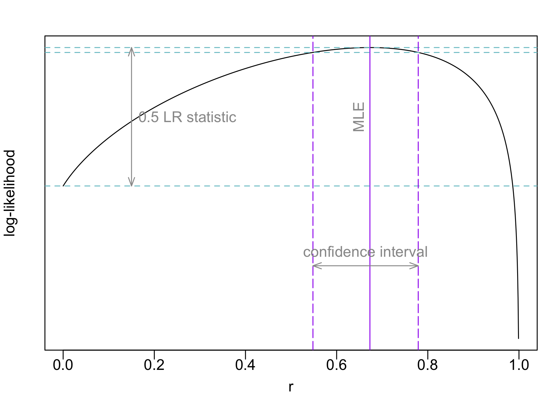
par(pardef)
![]()